Why is the [place software name here] so slow?
Such types of questions may hit a development team surprisingly, since a lot of software is being developed with blissful disregard for its performance and usage of resources. Especially if a software needs to perform a non safety critical function and performance is a lower priority to pure functionality. After all, doesn’t it only need to store and retrieve some data and render it in a UI? However, once the reality of a go-live hits, it usually comes with a growing amount of real-world users or data and software performance may suddenly become the most pressing matter in a project. A software that performs poorly may drive away users and profits, become unreliable or fail outright when it’s supposed to control processes or machines. Just as a poorly performing software wastes resources. Who wants to have their new mobile phone’s app drain the battery twice as fast after an update introduced performance issues? On a larger scale, inefficient software would waste resources of a data centers or server farms. Both in terms of energy and running cost.
But to identify application performance issues, an understanding of the most fundamental concepts of software performance is necessary. For those who haven’t had the opportunity to work on software performance before, this post aims to illustrate and provide an overview of the most fundamental concepts of evaluating software performance. We’ll explain the most important metrics, explore how they can be measured and what to watch out for when measuring and analyzing these metrics. Cloud hosted applications promise flexible performance due to the ability to scale horizontally, but they introduce additional complexities for measuring performance, on which we will touch as well. Since software performance characteristics cannot be described by a single metric measurement, but requires many measurements, we’ll proceed to show some basic, useful statistics that allow you to represent software performance using a few representative values.
Metrics
When a software doesn’t react immediately after some action was initiated, it might be described as “slow”. In order to exactly quantify what “slow” means and how “slow” a software is exactly, a more accurate description or analysis of the software performance characteristics are necessary. Does a UI respond sluggishly to input? Is a web request taking long or timing out? In order to verifiably and quantifiably improve software performance, its basic performance characteristics must be known and made measurable. While many different metrics may be defined to describe how a system performs, there are always three fundamental characteristics to consider – response time, throughput and resource utilization. They always influence each other and can be measured in different context and at different granularities – from internal software components responding to function calls, to a system comprised of a multitude of software and hardware components with transactions spanning multiple applications. Which context and granularity is chosen for a measurement depends on the question to be answered by the measurement. Further metrics may be defined to describe a system’s performance of course, from highly abstract considerations, e.g. the amount of generated sales or bounce rates of users, to the very low-level measurements like the number of calls of a specific function. But we’ll limit this blog to the three fundamental metrics, as they are characteristics of each system independently of its nature.
Response time
Response time is often the most prominent of the fundamental performance metrics. It is the time between initiating an action until the action is being completed. Whether it’s a button click, a function call or a web request, how quickly a software responds to input is an immediately perceivable aspect of its performance. Below the surface, the observed response time of a request is usually comprised of a number of activities requiring time to complete. In the following figure the potential composition of a response time when sending a request to a server based application is illustrated. At the left the request is sent, starting the timeline which finishes at the right. While the complete response time is marked as a green dotted line, the different blue sections of the upper line show which activities added up to the overall response time, including network delay, queueing time and the actual processing time itself.
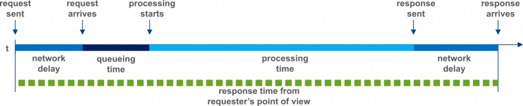
Response time composition.
Some care is required when analyzing response time, as the individual activities leading to the overall response time always depend on the context in which it is measured. A user browsing the internet may experience a very different response time when interacting with a Web UI than another application that runs on the same server as the web UI’s backend and directly sends requests to it. It is not just pure processing time that forms the response time, but also any time lost in network delays, spent on external application calls or on blocking wait times. Considering the context of a response time measure also becomes important when different types of requests result in very different processing times.
Throughput
Throughput becomes an important consideration as soon as processing of large amounts of data or requests is required. It describes how many requests a system processes in a given time frame.
Context is just as important for the throughput as for response time. Was throughput measured during times of high load, like requests to a food delivery application during lunch time? Or was it measured in the middle of the night, when the least requests were being processed. Which requests are being taken into account for a throughput measure is also of great importance, especially when analyzing an application’s behavior at the limit of its capacity, since some request types may be much more taxing than others, resulting in a lower maximum throughput.
Utilization
Response time and throughput are often quite visible characteristics of a system, but utilization of system resources impacts both, while being potentially much less visible. In the context of software, the most common resources are usually CPU, Memory, Storage and network. The use of these resources by a software system may be given as a percentage value and their usage may be modeled using queuing theory. On the most basic level, a queue consists of a processing resource and a waiting queue for things to be processed by this resource. The time between something being put into the queue and having been processed is the waiting time – or response time. Diving into queuing theory isn’t this article’s purpose, but details may be researched in the linked resources [wikipedia]. Queueing theory mathematically explains one particular property of queues: as the usage of the processing resource nears 100%, wait time increases. Unfortunately, the correlation between usage and waiting time is non-linear, forming a graph similar to below figure.
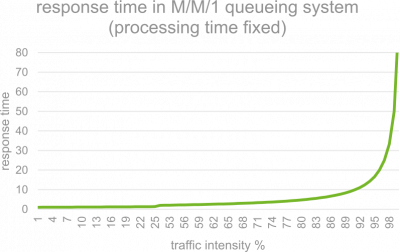
As a rule of thumb, usage of a given computing resource should therefore not exceed 75%-80%. Otherwise waiting times will increase rapidly, eventually leading to system failure. A typical malevolent example of such a scenario would be a denial of service attack.
Interplay of performance characteristics
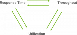
All three of the fundamental performance characteristics of a system may influence each other. Sometimes positively, but negative influence is just as possible. This influence may obscure the reason for an observed performance impact. Some such scenarios shall be illustrated in order to create an awareness for what needs to be considered, when analyzing a software’s performance.
Response time and throughput
As an example of the influence response time and throughput exercise on each other, let’s consider an (analogue) system we all hopefully use daily: A sink. A sink represents a simple system processing unit of „work“, in this case, draining water from a basin. The system capacity to store water for processing is the basin volume, its capacity for doing work in parallel is the sinks diameter and the processing time for a droplet – or molecule – of water, is the time it spends flowing through the drain. The system throughput is then the volume of water it is able to drain in a given amount of time, while its response time is the time it takes a water droplet between falling into the basin to coming out at the end of the sink. Ideally, our system would have a high capacity for processing parallel work, while also featuring a short processing time. However, one does not necessarily come with the other. On the other hand, once the system’s limits are approached, one may very well affect the other.
Let’s consider these two examples of different sinks:
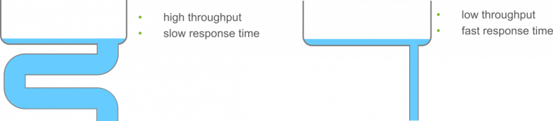
Given earth’s gravity and neglecting other factors, water will flow in all sinks at the same pace and only the sink’s length determines how long it takes, while only its diameter determines the throughout. A longer drain will mean a longer processing time and therefore a longer response time. The left example of a sink will reach a high throughput, since the sink’s diameter is large, but will have a long response time, since the sink is long and winded. The left example will have a short response time due to its short sink, but the maximum throughput is severely limited by the sinks diameter. This isn’t an issue, until more water starts arriving than can flow out at a time, meaning the “arrival rate” will exceed the system’s throughput.
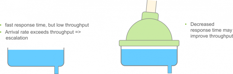
When that happens, the sink will start to look like in the following picture – it fills up. If the arrival rate keeps up, this will eventually result in system failure. The sink will overflow. Before that happens however, we’ll observe increasing response times, since the basin is already full and any water flowing into it, will most likely take a lot longer to be drained than it would if the basin was still empty. Here, a lack of throughput will eventually negatively affect response times.
It is however still possible to reach a high throughput, even for a system with a relatively low capacity for parallel work, if the processing time are simply very short. That way, more units of work may be processed in the same timeframe. Under the previous assumption of water flowing at a constant pace through the sink, that would be hard to model. But with a bit of creativity, it’s physically possible to speed up the “processing time” of the water: put it under pressure! The somewhat contrived contraption in the second illustration will help the pictured water draining system reach a higher throughput, despite a sink with a low diameter.
There is only one aspect of this analogous system, that will usually not transfer to a software system: A longer sink simultaneously increases the system’s capacity to contain water and the throughput stays constant. Software does not enjoy such a luxury when processing time for a single request in an application is increased. If the capacity for parallel requests is exhausted and processing time increases further, throughout will decrease.
Utilization vs. Response time and throughput
Utilization directly influences waiting times, which will have an impact on both response time and throughput – primarily negatively if utilization rises, however, either may influence utilization as well however. An unnecessarily processing heavy application will have higher response time for its functions than an optimized one and increased CPU usage as well. A higher throughput will as well lead to increased utilization of processing resources. Even in here however, scenarios exist in which the influence between the performance characteristics is not as obvious. A synchronous, blocking call to an external resource may stall an application thread for some time, resulting in a high response time. Utilization however, e.g. of the CPU, will remain low.
Performance characteristics in the cloud – not everything is as it seems
Migrating applications to a cloud-based deployment or developing them to be run in a cloud environment from the start has become a trend. It offers horizontal scalability of applications through adaptable clusters of application instances, vertical scalability through purchasing of higher end computing resources and therefore flexibility of hardware configuration, and promises to offload hardware complexity to the cloud provider. But all that convenience comes at a cost for performance concerns.
Response time and throughput of an application aren’t necessarily directly influenced if it’s deployed in the cloud, but estimations of resource utilization become a challenge. While metrics like CPU utilization, memory utilization and network I/O may be available, they must always be taken with a grain of salt due to the various levels of virtualization that may influence the application’s actual behavior. One important factor to consider is CPU steal time [cpu-steal-time]. A Virtual Machine’s scheduler may allocate processor time to your application, but the underlying OS’ hypervisor may be allocating the physical CPU’s time away to other VMs as well. As a result, processing tasks of the application may take longer despite the CPU’s utilization not appearing very high.
It’s therefore important to look closely at features and behavior of the cloud environment when analyzing performance of cloud-based applications. Aside from steal time as general factor in virtualized environments, the – usually useful – features offered by cloud providers may also turn out to mask performance issues. Consider non persistent and fast local SSD storage offered by Google. It may speed up I/O heavy tasks, but it doesn’t persist data after a cloud instance was stopped. If such an instance is re-initialized, the SSD storage may need to be filled with data at first, which can lead to an application performing differently than usual for a time after the cloud instance was initialized. Similarly a timely limited burst feature for CPU or IO, as available in some cloud instances (AWSEC2-ebs-io-characteristics, google-cloud-compute-machine-types) are helpful when coping with brief spikes in load. Should however a general increase of an application’s load happen to be the reason for the bursts being activated, it will overstay the burst. The then throttled CPU or IO resources may be faced with a much-increased load and utilization, in turn leading to additional slowdown and potentially failure of the application. At a glance it might appear that the application and environment were coping with an increased load just fine until the failure, when in fact the burst briefly changed the application’s performance characteristics. In such a scenario, performance optimizations and/or a more capable cloud instance may be required to cope with the now higher average load.
While the added complexity of a cloud-based environment may lead to unintuitive performance characteristics on the surface, closely inspecting the respective cloud instance features and analyzing an application’s performance with these features in mind will help identify the causes for potentially observed issues. In order to observe issues however, software performance should be measured, whether the application in question is deployed to the cloud, on a server or runs locally on a machine.
Measurement and statistics
A detailed description of how to measure software performance and collect metrics is out of scope for this article, but we’ll touch on some basic concepts to keep in mind and some helpful tools for collecting the needed information.
Performance Engineering Activities
Each measurement should be taken with the purpose of answering a question. What to measure, how to measure and when to measure depends on the question the measured values should answer and where a software is in its lifecycle. During the architecture and design phase, models and simulation enable to e.g. estimate required hardware configurations. At this point RETIT’s simulation toolchain may be of help. Once the application reaches the development and productive phase, three classes of tools especially help to collect general metrics and measurements: Monitoring and metrics tools like Prometheus and Graphite help to collect measurements and statistics. APM tools, like Dynatrace and AppDynamics or OpenTelemtry-based tools on the open source side allow to collect traces, but also statistics and metrics. Finally, test tools like JMeter, Gatling or Locust collect measurements throughout their tests, helping to analyze especially response times under test conditions.
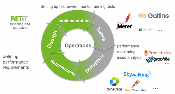
Performance engineering activities throughout the software life cycle and useful tools.
After measurements were made and many data points collected, some sense needs to be made of the collected data sets without investigating every single of the potentially thousands of data points individually. Therefore, the collected measurements ought to be aggregated to representative values. Many of the tools mentioned above are already capable of applying basic statistical methods to do such aggregation of test results and the two maybe most important statistics shall be introduced here.
Statistics
Many statistical values can be computed from collected metrics measurements, but often statistics are applied to aggregate many measurements into a “typical value”, representing all those values. The two probably most common statistical values used for this are the (arithmetic) mean and the median. The arithmetic mean is simply the sum of all collected values, divided by the amount of collected values. The median on the other hand is the 50th percentile. Slightly simplified this means when all collected values are ordered, it is the value in the exactly middle, or equal larger than one half and smaller or equal than the other half of all collected values. They each represent slightly different properties of a distribution and should therefore be considered together, not individually. The mean is biased towards outliers in the values, whereas the median tends to represent the majority of values better. Imagine a small town with ten inhabitants, nine of whom have a middle-class income. One however is Bill Gates. If only the mean was considered to represent the town’s population’s income, it would look as if this was a town of millionaires. The median however tells a different story: It would correspond to a middle-class wage, therefore representing most of the population, but giving no indication that there are extreme outliers. Together however, they allow to discern that the population mostly consists of middle-class workers, but there must be some extreme outliers, since the mean diverges significantly from the median. If the difference between mean and median was small on the other hand, it would indicate that there are not many or no extreme outliers.
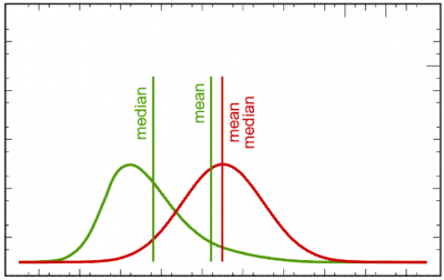
Mean and median for two different distributions (green/red).
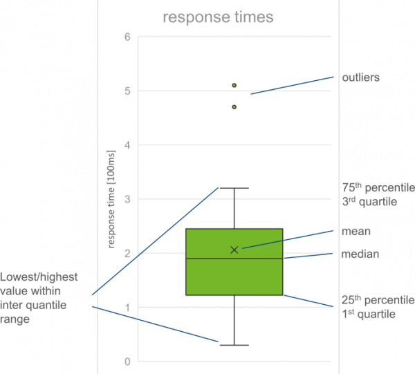
A concise visual way of presenting a large number of measurements is the box plot [wikipedia]. It conveys information about the distribution of a set of values along one axis. Where the majority of the distribution’s values are located, the a box is drawn. The box’s upper and lower end usually indicate the upper and lower quartiles, (i.e., the 25th and 75th percentiles). On either end of the box, whiskers will be drawn. Depending on the box plot’s variant, the whiskers may represent percentiles or maximal/minimal values. Likewise, maximum and minimum values may be represented outside of the whiskers as dots.
Conclusion
If you’re new to the topic of software performance, this article hopefully provided you with a helpful overview of the basic core concepts, both in general and in terms of the unexpected side effects one must look out for in a cloud environment. If you’re already familiar with the topic and still read on to this paragraph, you hopefully found a useful refresher and reference. Response time, throughput and utilization were introduced, being the three most fundamental performance metrics and characteristics of a software. Some exemplary interdependencies were presented and some of the less intuitive effects on these performance characteristics of deploying a software in a cloud environment were explored. Several ways and tools to collect measurements of the aforementioned performance metrics were named as well as the two statistics mean and median to aggregate the results into representative values and the box plot as a way of concisely visualizing a large set of collected data points.
If you’d like to review the performance of your software now with these fundamental concepts in mind, you might be looking for tools that help you collect metrics to use in your analysis. Perhaps our post on Open Source Application Performance Monitoring Tools can provide you with a helpful starting point. If you need support from one of our Software Performance Consultants to get you started on your performance journey, let us know!